This post is part of a series about machine learning and artificial intelligence. Click on the blog tag “huskyai” to see related posts.

• Overview: How Husky AI was built, threat modeled and operationalized
• Attacks: The attacks I want to investigate, learn about, and try out

The previous post covered some neat smart fuzzing techniques to improve generation of fake husky images.

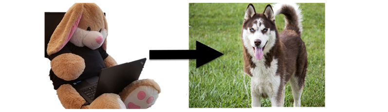
The goal of this post is to take an existing image of the plush bunny below, modify it and have the model identify it as a husky.

Let’s dive into it.

Calling the prediction API

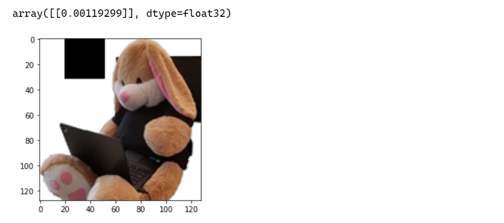
Running our plush Shadowbunny image through the prediction showed a much lower than 1% chance of it being a husky.

shadowbunny_image = load_image("shadowbunny.png")
predict(shadowbunny_image[0])["score"]

0.00038117

This looks good, certainly far from being seen as a husky by the system.

Let’s see what attacks we can come up with.

Testing ideas

To get started I will do some of my own research and experiments and then look at what more experienced researches have been doing. Here are some ideas:

1. Sliding block: Pick a 32x32 delta image and insert it into the picture. Possibly using a sliding window to see how much the prediction score changes. See how it changes the prediction score.
2. Sequential probing: Similar to the first idea, go over each pixel and change it to see how it impacts the score, keep those pixels that increase score (slow and lots of API calls). Repeat until prediction reaches 50%.
3. Randomly spraying pixels: Randomly add pixels to the image and if it increases the prediction score keep it if not try again. Repeat until prediction reaches 50%
4. Machine learning to optimize the delta image: Applying machine learning to “reverse optimize” the loss. Sort of gradient ascent. I assume that this is the best way of doing this, and that’s what adversarial machine learning researchers work on.

Those are the main ideas I had come up with and tested for, let’s look at how that went.

Test Case 1: Sliding block across image to find “hot spots”

The idea behind this is to possible find areas of the image that cause large changes in the prediction.

I went ahead to write some code to pick a couple of pixel blocks (32x32) of various colors and moved them in larger steps across the base image to see if any of those cause a larger change in prediction score.

Here is how this looks like in action:

You can see I even tried moving a small 32x32 pixel husky image over the Shadowbunny to try and trick the model.

The following pictures shows a good increase in prediction by using the black block:

In the end I took the best scores for each block (white, black, random, and a husky image block) and merged them all together in a final prediction which resulted in a score of 3.14%.

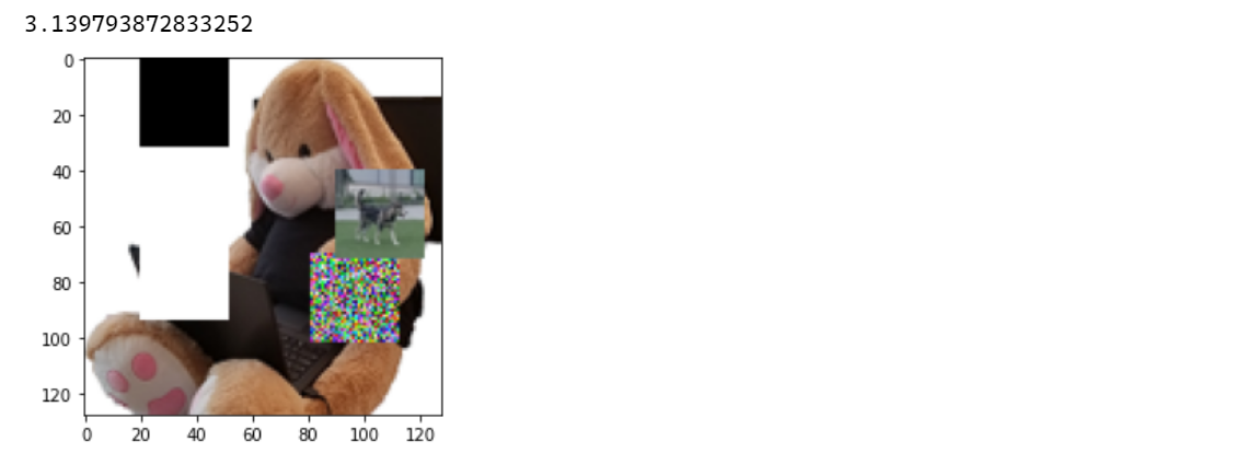
The idea is working but this is still far away from 50%…

And as can be seen in the screenshot above, the blocks are very visible on the Shadowbunny image.

Rate limiting shortcut

The drawback for the attacker (a good thing) is that these attacks create many queries to the model. With the current rate limiting in place I would wait for at least a day… Hence, I took a testing shortcut to bypass rate limiting. So, the code above is querying the model directly (not via the web endpoint).

An adversary can create and use their own model (that mimics ours) to do this, or just wait until the slow queries are done, or compromise the environment to get access to the model file (Assume Breach mindset). We will discuss such attacks in the future.

For now let’s focus on the perturbing pixels on the image to create an adversarial example.

Test Case 2: Sequential probing (keeping best ones)

The second idea was similar to the first one but with much smaller blocks. Additionally, it includes a feedback mechanism (technically making this some form of AI, haha) to only keep those pixels that actually increased the accuracy. The detailed steps are as follows:

1. Start at index 0,0 of the image and change pixel at that location
2. Run the image through a predict and record score
3. If the result is a new best_score, then store it
4. Take a larger step (4 pixels) to index 0,4 and update the pixel at that location again
5. Run the image through predict and record the score
6. If the result is a new best_score, then store it
7. And so forth until we either reach a best_score > 50% or we end at the bottom of the image.

The major drawback of this was that it creates a lot of queries. With rate limiting in place I would have to wait for a long time for this to finish. So, I took a shortcut here and tested this locally directly against the model, just to see if it might work.

Here is the code:

def find_best_pixels(image):

    attempts = 0
   
    initial_score = float(model.predict(image))
    
    step_size = 2
    block_size = 2
    delta_mid = np.ones([1, block_size,block_size, 3]) * 128/255.

    best_score = 1e-100
    best_image = 0

    run_image = image

    #experimented a bit with the starting row, lower half (row 70) was good
    for i in range(70, NUM_PX-block_size+1, step_size):
        
        for j in range(0, NUM_PX-block_size+1,step_size):
            
            temp_image = np.copy(run_image)
            temp_image[0, i:i+block_size, j:j+block_size] = delta_mid

            current_score = float(model.predict(temp_image)[0][0])
            attempts = attempts + 1 

            if current_score > best_score:
                best_score = float(current_score)
                run_image = temp_image

            if best_score > 0.5:
                return run_image
    
            #also update image every row
            plt.imshow(run_image[0], interpolation='nearest')
            plt.text(y=10, x=150, s=f"Initial Score: {initial_score:8f}", fontsize=12)
            plt.text(y=20, x=150, s=f"Best Score:   {best_score:8f}", fontsize=12)
            plt.text(y=30, x=150, s=f"Current Score: {current_score:8f}", fontsize=12)
            plt.text(y=40, x=150, s=f"API Call Count: {attempts}", fontsize=12)
            plt.show()
            clear_output(wait=True)  

image = load_image("shadowbunny.png")
best_image = find_best_pixels(image) 

To my surprise it works! :)

Although it requires about 800-5000+ calls to the API depending on block_size and step_size. Also, the color of the pixel makes a big difference.

What other options are there?

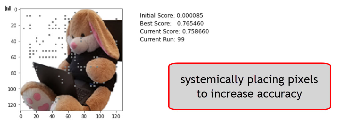
Test Case 3: Randomly spraying pixels (keeping best ones)

The next idea was to randomly put pixels on the image, and keeping those that improve the score. The following animation shows the attack in progress and you can see that we reach a score of 50%+ was reached this way.

Nice!

It took 451 calls to the API, which is not that bad I thought and doable with the current rate limiting within a few hours.

For completeness, here are the core pieces of code for the third scenario:

def find_best_pixels_random(image):

    initial_score = float(model.predict(image))
    
    block_size = 1
    delta_mid = np.ones([1, block_size,block_size, 3]) #* 128/255.

    best_score = 1e-100
    best_image = 0

    run_image = image

    for count in range(4000):
            
        i = np.random.randint(0,128-block_size)
        j = np.random.randint(0,128-block_size)

        temp_image = np.copy(run_image)
        temp_image[0, i:i+block_size, j:j+block_size] = delta_mid * 0#(np.random.randint(200,256)/25.)

        current_score = float(model.predict(temp_image)[0][0])
        attempts = attempts + 1 

        if current_score > best_score:
            best_score = float(current_score)
            run_image = temp_image

        if best_score > 0.5:
            return run_image

        #update image so we see a nice animation
        plt.imshow(run_image[0], interpolation='nearest')
        plt.text(y=10, x=150, s=f"Initial Score: {initial_score:8f}", fontsize=12)
        plt.text(y=20, x=150, s=f"Best Score:   {best_score:8f}", fontsize=12)
        plt.text(y=30, x=150, s=f"Current Score: {current_score:8f}", fontsize=12)
        plt.text(y=40, x=150, s=f"API Call Count: {attempts}", fontsize=12)
        plt.show()
        clear_output(wait=True)  

image = load_image("shadowbunny.png")
best_image = find_best_pixels_random(image) 

Next, I want to explore what TensorFlow offers in this regards. There is also a library called Cleverhans - that I will post about at a later point.

Test Case 4: Using ML to optimize adversarial images

There are more advanced ways of doing such perturbation attacks. The most famous/popular method seems to be Fast Gradient Signing Method (FSGM). The method is described in detail this paper called Explaining and Harnessing Adversarial Examples .

While learning more about this I ran across this talk Adversarial Robustness - Theory and Practice by J. Zico Kolter and Aleksander Madry. That talks is a must watch if you want to learn more about this.

Here are some other good resources to learn more about these techniques:

• Adversarial ML Tutorial Site
• Adversarial Examples in Deep Learning
• TensorFlow documentation of FGSM

To be most efficient the adversary has to either have access to the model or use a model that is similar. From the FGSM paper:

An intriguing aspect of adversarial examples is that an example generated for one model is often misclassified by other models, even when they have different architectures or were trained on dis-joint training sets.

Threat modeling already identified the adversary gainin gread access to the model (e.g. “model stealing”), so we will research that attack in a future post. I can think of least two ways that I already can think of, but for now let’s continue to assume we have a model file again.

Here is the code used to generate an adversary example via an Adam optimizer:

shadowbunny = load_image("shadowbunny.png")
initial_score = model.predict(shadowbunny)

image_tensor = tf.constant(shadowbunny, dtype=tf.float32)
delta        = tf.Variable(tf.zeros_like(image_tensor), trainable=True)
optimizer    = tf.keras.optimizers.Adam(learning_rate=0.0008)
loss_object  = tf.keras.losses.BinaryCrossentropy()

best_score = 0
candidate  = 0

for round in range(40):
    with tf.GradientTape() as tape:
        tape.watch(image_tensor)
        
        candidate = image_tensor + delta
        candidate = tf.clip_by_value(candidate, clip_value_min=0, clip_value_max=1)    

        best_score = model(candidate)
        loss_value = loss_object( tf.convert_to_tensor([1]),  tf.convert_to_tensor(best_score))
        
        #update image every iteration for a nice animation
        clear_output(wait=True)  
        plt.imshow(candidate[0])
        plt.text(y=10, x=150, s=f"Initial Score: {initial_score[0][0]:8f}", fontsize=12)
        plt.text(y=20, x=150, s=f"Best Score: {best_score[0][0]:8f}", fontsize=12)
        plt.text(y=30, x=150, s=f"Current Loss: {loss_value:8f}", fontsize=12)
        plt.show()
        
    gradients = tape.gradient(loss_value, image_tensor)
    optimizer.apply_gradients([(gradients, delta)])
    
print("Final Score: ", best_score.numpy()[0][0])

Below is an animation that shows the running attack. Pay attention to the pixels of the image. Do you notice some of them are slightly changing especially towards the final rounds?

For reference here is the final adversarial example. Look at the white areas on the upper left. You can see slight changes colors. Quite subtle, but they are visible:

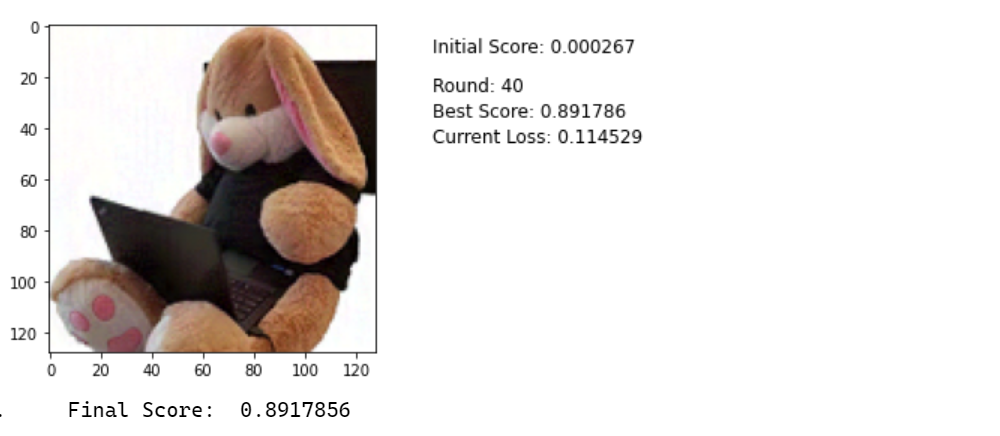
Using this technique, I got a nearly 90% accuracy with just 40 iterations. By increasing the learning rate this can be further reduced.

Pretty impressive.

What’s next?

This and the previous blog posts show that machine learning is fragile and brittle.

I hope you enjoyed reading and learning about this as much as I do. Next will be stealing and backdooring models. Stay tuned!

If you find this interesting, follow me on Twitter: @wunderwuzzi23.

Cheers.

Appendix

These are the core ML threats for Husky AI that were identified in the threat modeling session so far and that I want to research and build attacks for.

Links will be added when posts are completed over the next serveral weeks/months.

1. Attacker brute forces images to find incorrect predictions/labels
2. Attacker applies smart ML fuzzing to find incorrect predictions
3. Attacker performs perturbations to misclassify existing images (this post)
4. Attacker gains read access to the model - Exfiltration Attack
5. Attacker modifies persisted model file - Backdooring Attack
6. Attacker denies modifying the model file - Repudiation Attack
7. Attacker poisons the supply chain of third-party libraries
8. Attacker tampers with images on disk to impact training performance
9. Attacker modifies Jupyter Notebook file to insert a backdoor (key logger or data stealer)
10. Attacker uses Generative Adversarial Networks to create fake husky images

References

• Adversarial Robustness - Theory and Practice (NeurIPS 2018 Tutorial)
• TensorFlow Adversarial FGSM
• Explaining and Harnessing Adversarial Examples
• Adversarial Examples in Deep Learning