Husky AI: Building a machine learning system
This post is part of a series about machine learning and artificial intelligence.
In the previous post we described the overall machine learning pipeline.
In this post we dive into the technical details on how I built and trained the machine learning model for Husky AI.
After reading this you should have a good understanding around the technical steps involved in building a machine learning system, and also some thoughts around what can be attacked.
Part 2 - Building the model
Building a machine learning model is a very iterative process and takes a while.
Initially I started without TensorFlow and built a neural network, forward and backpropagation algorithms in Python. This is basically what the Machine Learning and deeplearning.ai courses I took teach you to do. I liked this as it gives a good understanding on what is going on under the hood.
The first step is gathering training data - images in the case of building Husky AI.
Gathering training and validation data
To gather training data for husky and non-husky images I used Bing to gather images and did some manual data cleansing. It was about 1300 husky images and 3000 random other ones, including other dogs, people, and other objects.
I used Bing’s image search to gather images. Check out Azure Cognitive Services and Bing Image Search. They offer a free API to search and download images, all you must do is create an Azure account (which is also free) and then you can request an API key.
Source code to Azure Cognitive Services (Bing Image Search)
I published code to call the Bing search API here if you are interested to try it also.
Training and validation data
Images are typically stored in dedicated folders for training and validation sets, and according to there label. This makes it easier later on because ML frameworks can use the “folder name” as the label for images. This is one of these typically pre-processing steps, where we get all the ducks, aehm, huskies in a row.
For instance, I have the following directory structure for images:
   data/training/husky
   data/training/nothusky
   data/validation/husky
   data/validation/nothusky
In machine learning data is split into separate sets. There are folders for training data and validation data. This is needed because we do not want to train our model on validation or test data. Validation and test data are used to tell us how well the model is performing on images not seen before.
Attack idea: Attacker can attempt to poison either set of images, which can lead to vastly different results.
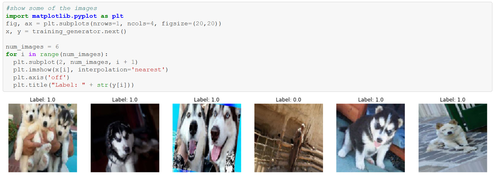
Exploring the images
Building the model
The first model I built had only one layer and was basically just doing what is called “logistic regression” with a binary classifier.
It gave about a 62% accuracy, which I thought was good already. Although, I wanted to apply more of the knowledge I was learning from Andrew Ng’s class and played around with a lot of different and more complex variations. Including regularization, convolutions, dropouts and things along those lines.
In the end I ended up with a convolutional neural network (CNN) with the following layout.
model = tf.keras.models.Sequential([
    tf.keras.layers.Conv2D(32, (3,3), activation="relu", input_shape=(num_px, num_px, 3)),
    tf.keras.layers.MaxPooling2D(2, 2),
    tf.keras.layers.Dropout(0.4),

    tf.keras.layers.Conv2D(64, (3,3), activation="relu", input_shape=(num_px, num_px, 3)),
    tf.keras.layers.MaxPooling2D(2, 2),

    tf.keras.layers.Dropout(0.4),

    tf.keras.layers.Conv2D(128, (3,3), activation="relu"),
    tf.keras.layers.MaxPooling2D(2,2),
    tf.keras.layers.Dropout(0.4),

    tf.keras.layers.Flatten(),
    tf.keras.layers.Dense(128, activation="relu"),
    tf.keras.layers.Dense(1, activation="sigmoid")
])

opt = tf.keras.optimizers.Adam(learning_rate=0.0005)
model.compile(optimizer=opt, loss="binary_crossentropy", metrics=["accuracy"])
For the optimizer I played around with RMSProp, but decided on Adam eventually. Here is a summary of the deep neural network that I’m using at the moment:
>> model.summary()

Model: "sequential"
_________________________________________________________________
Layer (type)                 Output Shape              Param #
=================================================================
conv2d (Conv2D)              (None, 126, 126, 32)      896
_________________________________________________________________
max_pooling2d (MaxPooling2D) (None, 63, 63, 32)        0
_________________________________________________________________
dropout (Dropout)            (None, 63, 63, 32)        0
_________________________________________________________________
conv2d_1 (Conv2D)            (None, 61, 61, 64)        18496
_________________________________________________________________
max_pooling2d_1 (MaxPooling2 (None, 30, 30, 64)        0
_________________________________________________________________
dropout_1 (Dropout)          (None, 30, 30, 64)        0
_________________________________________________________________
conv2d_2 (Conv2D)            (None, 28, 28, 128)       73856
_________________________________________________________________
max_pooling2d_2 (MaxPooling2 (None, 14, 14, 128)       0
_________________________________________________________________
dropout_2 (Dropout)          (None, 14, 14, 128)       0
_________________________________________________________________
flatten (Flatten)            (None, 25088)             0
_________________________________________________________________
dense (Dense)                (None, 128)               3211392
_________________________________________________________________
dense_1 (Dense)              (None, 1)                 129
=================================================================
Total params: 3,304,769
Trainable params: 3,304,769
Non-trainable params: 0
If you are not familiar with neural networks these layer names might seem a bit mystical. To understand this in more detail, I recommend looking at my previous post for some good learning material.
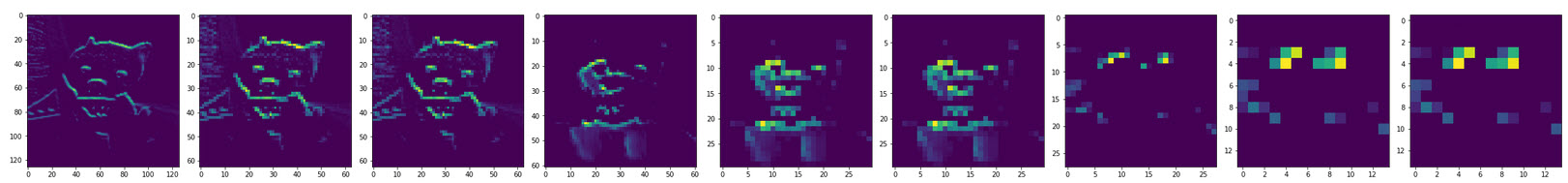
Convolutions
One thing to highlight is the use of convolutions in neural network (especially for image processing). Convolutions are a technique to apply filters to an image and as a result it makes neurons “see” specific features.
As an example, below you can see images while it goes through some of the hidden layers of the neural network. You can see in the how the convolutions seem to be focused on highlighting the ears of a husky. This is something specific the neural network now uses to figure out if the image contains a husky or not - pointy ears!
So much about the layout of the neural network itself.
Training the model
Training the model with Keras is pretty straight forward and is done via model.fit (or model.fit_generator respectively).
history = model.fit_generator(training_generator,
                              epochs=200,
                              steps_per_epoch=80,
                              validation_data=validation_generator,
                              validation_steps=20,
                              callbacks=[callbacks],
                              verbose=1)
- Input Training and Validation Data: I used generators for training and validation sets because I was loading images from the hard drive via an API called
flow_from_directory. More about that a bit further down. - Epochs: Other parts to specify are the training duration (number of epochs and steps).
- Callbacks: Passing a callback to the
fitfunction allows to observe the training in more detail - in my case I used it to stop training when reaching a certain accuracy.
The definition of the callback looks like this:
DESIRED_ACCURACY = 0.99

class myCallback(tf.keras.callbacks.Callback):
  def on_epoch_end(self, epoch, logs={}):
    if(logs.get("accuracy") > DESIRED_ACCURACY):
      print(f"\nReached {DESIRED_ACCURACY}% accuracy - cancelling training.")
      self.model.stop_training = True

callbacks = myCallback()
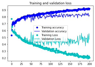
After training for a few hours, the model had an accuracy on the validation set in the mid 70% range. Not bad, and I still wanted to apply Image Augmentation which I had just learned about in the deeplearning.ai course.
Image Augmentation
Since my training set was rather smaller, I used a technique called Image Augmentation. Image Augmentation means that when training the model, the images feed to the model are updated on the fly. For instance, they are cropped, or flipped and things like that. This is to increase the training set and provide more variations. I thought that is a pretty neat trick.
I updated and played around with different algorithms, model structures as well as performing image augmentation. In TensorFlow this is done with the ImageDataGenerator and flow_from_directory.
training_datagen =  ImageDataGenerator(
    rescale=1/255,
    shear_range=0.2,
    zoom_range=0.2,
    rotation_range=30,
    fill_mode="nearest",
    horizontal_flip=True)

training_generator = training_datagen.flow_from_directory(
    training_folder,
    target_size=(num_px, num_px),
    batch_size=batch_size,
    class_mode='binary')
By using Image Augmentation the model landed a ~84% accuracy on the validation set after a few hours of training.
Saving the model
In Keras a model is saved with a call to .save. This includes the model structure and the weights.
model.save("huskymodel.h5")
There is also the API to only store the weights, called .save_weights. In that case you have to manually construct the model before loading the weights again. This is useful for saving checkpoints during training for instance.
In TensorFlow there are two file formats to choose from when saving models .h5, and also a SaveModel. For now we will just focus on the .h5 file format.
Attack idea: As you can image the model file itself is a pretty high value asset. It does contain both the layout of the neural network, as well as the model weights. Tampering with this file will allow to add backdoors and cause a lot of other issues. We will analyze this more during threat modeling.
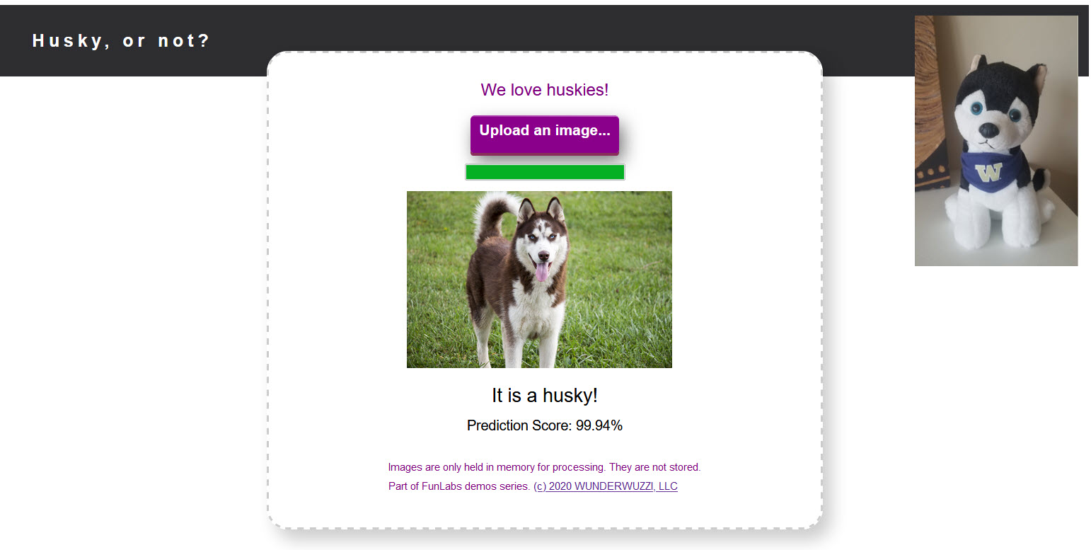
Performing predictions
To perform a prediction we load an image into memory and pass it to the model with model.predict.
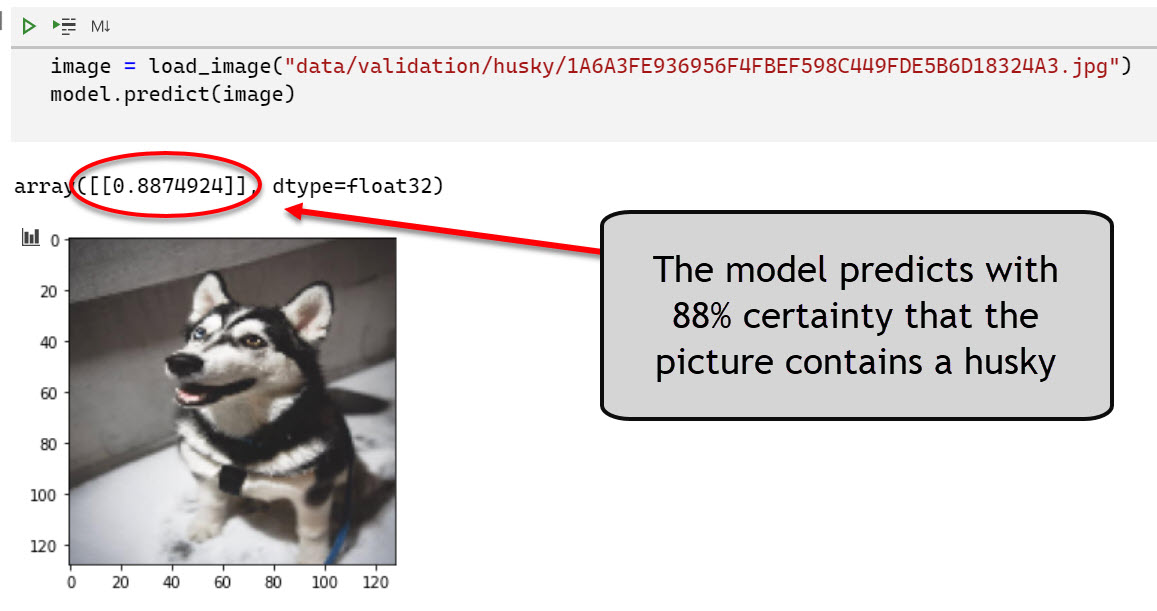
The model can still benefit from improvements (such as transfer learning, where we build on the shoulders of other more powerful pre-trained models). It has an accuracy of a bit over 80% on the validation data - which is okay for now.
What’s next?
Hopefully this was useful to get a better understanding around the moving bits and pieces involved in building a ML application. Next we will dive into the aspects of MLOps and we discusshow to operationalize the model and put it behind a web application and make it available to end users.
Twitter: @wunderwuzzi23